大模型从零开始（二）手撕代码

{% quot 本文部分内容整理自网络和 ChatGPT，侵删/仅供参考。 %}

Shuffle 函数

import random
def shuffle(nums):
	for i in range(len(nums) - 1, 0, -1):
		j = random.randint(0, i)
		nums[i], nums[j] = nums[j], nums[i]
	return nums

Softmax 函数

处理数值稳定性。

$softmax (x_{i}) = \frac{e ^{x_{i}}}{\sum _{j = 1}^{n} e ^{x_{j}}}$

import numpy as np
def softmax(logits: np.ndarray) -> np.ndarray:
    # 减去最大值以提高数值稳定性，对结果相当于分子分母同时约简了exp(max)
    max_logits = np.max(logits)
    exp_logits = np.exp(logits - max_logits)
    return exp_logits / np.sum(exp_logits)
 
# 示例用法
logits = np.array([2.0, 1.0, 0.1])
softmax_values = softmax(logits)
print(softmax_values)  # 输出 softmax 概率
 
def softmax(input_tensor, dim):
    # 数值稳定性处理：减去最大值防止溢出
    max_vals = torch.max(input_tensor, dim=dim, keepdim=True).values
    exp_x = torch.exp(input_tensor - max_vals)  # 减去最大值后做指数运算
    sum_exp = exp_x.sum(dim=dim, keepdim=True)  # 沿指定维度求和，保持维度
    return exp_x / sum_exp  # 广播机制自动对齐维度

更简洁的处理数值稳定性方案实现： $lo g softmax (x_{i}) = x_{i} - max (x) - lo g (\sum_{j = 1}^{n} e^{x_{j} - m a x (x)})$

import numpy as np
 
def log_softmax(scores: list) -> np.ndarray:
    # Subtract the maximum value for numerical stability
    scores = scores - np.max(scores)
    return scores - np.log(np.sum(np.exp(scores)))

MSE 损失

import numpy as np
def mean_squared_error(y_true: np.ndarray, y_pred: np.ndarray) -> float:
    # 确保输入为 NumPy 数组
    y_true = np.asarray(y_true)
    y_pred = np.asarray(y_pred)
    # 计算 MSE
    mse = np.mean((y_true - y_pred) ** 2)
    return mse
 
# 示例用法
y_true = [3, -0.5, 2, 7]
y_pred = [2.5, 0.0, 2, 8]
mse_value = mean_squared_error(y_true, y_pred)
print(f"均方误差: {mse_value}")

另外，更完整的场景参见具有反向传播的单神经元

交叉熵损失

$H (p, q) = - \frac{1}{N} \sum_{i = 1}^{N} p (i) l o g (q (i))$

# powered by ChatGPT4o
import numpy as np
def binary_cross_entropy(y_true: np.ndarray, y_pred: np.ndarray) -> float:
    # 确保预测值在有效范围内，避免log(0)
    y_pred = np.clip(y_pred, 1e-15, 1 - 1e-15)
    # 计算交叉熵损失
    loss = -np.mean(y_true * np.log(y_pred) + (1 - y_true) * np.log(1 - y_pred))
    return loss
 
# 示例用法
y_true = np.array([1, 0, 1])
y_pred = np.array([0.9, 0.1, 0.8])
loss_value = binary_cross_entropy(y_true, y_pred)
print(f"二分类交叉熵损失: {loss_value}")
 
# 二分类不用MSE：CE更符合概率分布的实质（熵）、以及sigmod或softmax是对类的概率进行估计，所以在计算损失时天然适应概率意义上的相近，而非欧拉距离上的相近。同时MSE无差别地关注全部类别上预测概率和真实概率的差，交叉熵关注的是正确类别的预测概率，所以相当于MSE引入了一个先验即所有类别的损失贡献是等价的。
 
def categorical_cross_entropy(y_true, y_pred):
    """
    计算多分类交叉熵
    :param y_true: 真实标签，独热编码形式的 numpy 数组，形状为 (样本数, 类别数)
    :param y_pred: 模型预测的概率分布，形状为 (样本数, 类别数)
    :return: 每个样本的交叉熵损失值
    """
    # 避免对数计算中的数值不稳定，加上一个小的 epsilon 值
    epsilon = 1e-12
    y_pred = np.clip(y_pred, epsilon, 1. - epsilon)
    # 按公式计算交叉熵
    cross_entropy = -np.sum(y_true * np.log(y_pred), axis=1)
    return cross_entropy
 
# 示例数据
y_true = np.array([[1, 0, 0], [0, 1, 0], [0, 0, 1]])  # 独热编码标签
y_pred = np.array([[0.7, 0.2, 0.1], [0.1, 0.8, 0.1], [0.1, 0.3, 0.6]])  # 模型预测的概率
# 计算交叉熵损失
loss = categorical_cross_entropy(y_true, y_pred)
print("平均交叉熵损失:", np.mean(loss))

numpy 手撕二分类交叉熵全流程实现。

import numpy as np
def sigmoid(z):
	return 1 / (1 + np.exp(-z))
def sigmoid_derivative(z):
	return sigmoid(z) * (1 - sigmoid(z))
class SimpleNN:
	def __init__(self, input_size, hidden_size, output_size):
		self.weights1 = np.random.randn(input_size, hidden_size)
		self.bias1 = np.zeros((1, hidden_size))
		self.weights2 = np.random.randn(hidden_size, output_size)
		self.bias2 = np.zeros((1, hidden_size))
	def forward(self, X):
		self.Z1 = np.dot(X, self.weights1) + self.bias1
		self.A1 = sigmoid(self.Z1)
		self.Z2 = np.dot(self.A1, self.weights2) + self.bias2
		self.A2 = sigmoid(self.Z2)
		return self.A2
	def backward(self, X, y, lr):
		m = X.shape[0]
		# 输出层
		dZ2 = self.A2 - y
		dW2 = np.dot(self.A1.T, dZ2) / m
		db2 = np.sum(dZ2, axis=0, keepdims=True) / m
		# 隐藏层
		dA1 = np.dot(dZ2, self.weights2.T)
		dZ1 = dA1 * sigmoid_derivative(self.Z1)
		dW1 = np.dot(X.T, dZ1) / m
		db1 = np.sum(dZ1, axis=0, keepdims=True) / m
		# 更新权重
		self.weights1 -= lr * dW1
		self.bias1 -= lr * db1
		self.weights2 -= lr * dW2
		self.bias2 -= lr * db2
	def compute_loss(self, X, y):
		# 计算交叉熵损失
		A2 = self.forward(X)
		m = X.shape[0]
		loss = -np.mean(y * np.log(A2) + (1 - y) * np.log(1 - A2))
		return loss
	def train(self, X_train, y_train, epochs, lr):
		for epoch in range(epochs):
			self.forward(X_train)
			self.backward(X_train, y_train, lr)
			if epoch % 100 == 0:
				loss = self.compute_loss(X_train, y_train)
				print(f"Epoch:{epoch}/{epochs}, Loss: {loss:.4f}")
	def predict(self, X):
		A2 = self.forward(X)
		return (A2 > 0.5).astype(int)

交叉熵和 softmax 的组合求导非常优雅，仅是预测概率和真实标签之间的差异，优化方向符合直觉，并且计算极其简洁。另外，困惑度的计算也是和交叉熵相关的。

$Perplexity (P) = 2^{H (P, Q)}$ 在语言模型中，为确保一致，通常使用自然对数 $e$ 为底，困惑度 PPL 的原始定义是 $2$ 为底，整体不影响趋势分析。困惑度为 1 表示完全确定准确，最优状态，最差状态是无穷大，均匀分布时等于词表大小。总的来说，困惑度更适合在给定数据集的情况下评定语言模型的好坏，尤其适合风格迁移任务，例如让它尽可能输出格式符合百科的用语。而使用困惑度评价不同文本质量存在争议，因为常见但无聊的句子往往能够得到更低的困惑度，所以仅在没有参考文本的情况下才能有限选用。

max_length = model.config.n_positions
stride = 512
seq_len = encodings.input_ids.size(1)

nlls = []
prev_end_loc = 0
for begin_loc in tqdm(range(0, seq_len, stride)):
    end_loc = min(begin_loc + max_length, seq_len)
    trg_len = end_loc - prev_end_loc  # may be different from stride on last loop
    input_ids = encodings.input_ids[:, begin_loc:end_loc].to(device)
    target_ids = input_ids.clone()
    target_ids[:, :-trg_len] = -100

    with torch.no_grad():
        outputs = model(input_ids, labels=target_ids)
        # loss is calculated using CrossEntropyLoss which averages over valid labels
        # N.B. the model only calculates loss over trg_len - 1 labels, because it internally shifts the labels
        # to the left by 1.
        neg_log_likelihood = outputs.loss

    nlls.append(neg_log_likelihood)

    prev_end_loc = end_loc
    if end_loc == seq_len:
        break
        
ppl = torch.exp(torch.stack(nlls).mean())

多头注意力机制 (MHA)

import torch
import torch.nn as nn
 
class MultiHeadAttention(nn.Module):
	def __init__(self, num_heads, d_model, batch_size, seq_len):
		super(MultiHeadAttention, self).__init__()
		self.num_heads = num_heads
		self.head_dim = d_model // num_heads
		self.q_proj = nn.Linear(d_model, d_model)
		self.k_proj = nn.Linear(d_model, d_model)
		self.v_proj = nn.Linear(d_model, d_model)
		self.o_proj = nn.Linear(d_model, d_model)
	
	def split(self, x, batch_size):
		# 维度切分，(batch_size, seq_len, d_model) -> (batch_size, seq_len, num_heads, head_dim)
		x = x.view(batch_size, -1, self.num_heads, self.head_dim)
		# 重排维度，便于后续计算方便和并行多头
		return x.permute(0, 2, 1, 3)
 
	def forward(self, hidden_state, attention_mask=None):
		batch_size = hidden_state.size()[0]
		query = self.q_proj(hidden_state)
		key = self.k_proj(hidden_state)
		value = self.v_proj(hidden_state)
		query, key, value = self.split(query, batch_size), self.split(key, batch_size), self.split(value, batch_size)
		attention_scores = torch.matmul(query, key.transpose(-1, -2) / torch.sqrt(torch.tensor(self.head_dim)))
		if attention_mask is not None:
			attention_scores = attention_scores.masked_fill(attention_mask == 0, float('-inf'))
		# attention_scores、attention_probs 均为 (batch_size, num_heads, seq_len, seq_len)
		attention_probs = torch.softmax(attention_scores, dim=-1)
		output = torch.matmul(attention_probs, value)
		# output: (batch_size, seq_len, d_model)
		# contiguous: 确保张量内存中连续，确保view操作正常进行，一般均连续，permute和transpose操作可能改变
		output = output.permute(0, 2, 1, 3).contiguous().view(batch_size, -1, self.head_dim * self.num_heads)
		output = self.o_proj(output)
		return output

查询注意力机制 (MQA)

# powered by ChatGPT4o
import torch
import torch.nn as nn
import math
 
class MultiQueryAttention(nn.Module):
    def __init__(self, num_heads, d_model):
        super(MultiQueryAttention, self).__init__()
        self.num_heads = num_heads
        self.head_dim = d_model // num_heads
        assert d_model % num_heads == 0, "d_model must be divisible by num_heads"
 
        # Linear layers for Query, Key, Value
        self.q_proj = nn.Linear(d_model, d_model)
        self.k_proj = nn.Linear(d_model, self.head_dim)  # Shared Key for all heads
        self.v_proj = nn.Linear(d_model, self.head_dim)  # Shared Value for all heads
        # Output linear layer
        self.o_proj = nn.Linear(d_model, d_model)
 
    def forward(self, hidden_state, attention_mask=None):
        batch_size, seq_len, d_model = hidden_state.size()
        # Linear projections to create Query, Key, Value
        query = self.q_proj(hidden_state)  # Shape: (batch_size, seq_len, d_model)
        key = self.k_proj(hidden_state)    # Shape: (batch_size, seq_len, head_dim)
        value = self.v_proj(hidden_state)  # Shape: (batch_size, seq_len, head_dim)
        # Reshape Query for multi-head attention
        query = query.view(batch_size, seq_len, self.num_heads, self.head_dim).permute(0, 2, 1, 3)  # (batch_size, num_heads, seq_len, head_dim)
        # Reshape Key and Value for broadcasting
        key = key.unsqueeze(1).expand(-1, self.num_heads, -1, -1)  # (batch_size, num_heads, seq_len, head_dim)
        value = value.unsqueeze(1).expand(-1, self.num_heads, -1, -1)  # (batch_size, num_heads, seq_len, head_dim)
        # Scaled dot-product attention
        scale = 1 / math.sqrt(self.head_dim)
        attention_scores = torch.matmul(query, key.transpose(-1, -2)) * scale  # (batch_size, num_heads, seq_len, seq_len)
        if attention_mask is not None:
            attention_scores = attention_scores.masked_fill(attention_mask == 0, float('-inf'))
        attention_probs = torch.softmax(attention_scores, dim=-1)  # (batch_size, num_heads, seq_len, seq_len)
        # Weighted sum of Value
        context = torch.matmul(attention_probs, value)  # (batch_size, num_heads, seq_len, head_dim)
        # Concatenate heads and project output
        context = context.permute(0, 2, 1, 3).contiguous().view(batch_size, seq_len, -1)  # (batch_size, seq_len, d_model)
        output = self.o_proj(context)  # (batch_size, seq_len, d_model)
        return output

分组查询注意力机制 (GQA)

import torch
import torch.nn as nn
 
class GroupedQueryAttention(nn.Module):
	def __init__(self, num_heads, d_model, num_groups):
		super(GroupedQueryAttention, self).__init__()
		self.num_heads = num_heads
		self.head_dim = d_model // num_heads
		self.num_groups = num_groups
		self.each_group_count = num_heads // num_groups
		self.group_dim = self.head_dim * self.num_groups
		self.q_proj = nn.Linear(d_model, d_model)
		self.k_proj = nn.Linear(d_model, self.group_dim)
		self.v_proj = nn.Linear(d_model, self.group_dim)
		self.o_proj = nn.Linear(d_model, d_model)
		self.scaler = 1 / math.sqrt(self.head_dim)
 
	def kv_expand(self, x, batch_size, seq_len):
		x = x.view(batch_size, seq_len, self.num_groups, self.head_dim)
		x = x.unsqueeze(3).expand(-1, -1, -1, self.each_group_count, -1)
		x = x.reshape(batch_size, seq_len, self.num_heads, self.head_dim)
		x = x.permute(0, 2, 1, 3)
		return x
 
	def forward(self, hidden_state, attention_mask=None):
		batch_size, seq_len = hidden_state.size()[0], hidden_state.size()[1]
		query = self.q_proj(hidden_state)
		key = self.k_proj(hidden_state)
		value = self.v_proj(hidden_state)
		# 主要差异在下面两行
		query = query.view(batch_size, -1, self.num_heads, self.head_dim).permute(0, 2, 1, 3)
		key, value = self.kv_expand(key, batch_size, seq_len), self.kv_expand(value, batch_size, seq_len)
		attention_scores = torch.matmul(query, key.transpose(-1, -2)) / self.scaler
		if attention_mask is not None:
			attention_scores = attention_scores.masked_fill(attention_mask == 0, float('-inf'))
		attention_probs = torch.softmax(attention_scores, dim=-1)
		output = torch.matmul(attention_probs, value)
		output = output.permute(0, 2, 1, 3).contiguous().view(batch_size, -1, self.head_dim * self.num_heads)
		output = self.o_proj(output)
		return output

交叉注意力机制

该函数接受编码器的输出和查询 (query）作为输入，并返回注意力加权的编码器输出。

# powered by ChatGPT4o
import torch
import torch.nn as nn
 
class CrossAttention(nn.Module):
    def __init__(self, num_heads, d_model):
        super(CrossAttention, self).__init__()
        self.num_heads = num_heads
        self.head_dim = d_model // num_heads
        assert d_model % num_heads == 0, "d_model must be divisible by num_heads"
        self.q_proj = nn.Linear(d_model, d_model)  # 用于查询
        self.k_proj = nn.Linear(d_model, d_model)  # 用于键
        self.v_proj = nn.Linear(d_model, d_model)  # 用于值
        self.o_proj = nn.Linear(d_model, d_model)  # 最终输出
        
    def split(self, x, batch_size):
        # 维度切分，(batch_size, seq_len, d_model) -> (batch_size, seq_len, num_heads, head_dim)
        x = x.view(batch_size, -1, self.num_heads, self.head_dim)
        # 重排维度，便于多头并行计算
        return x.permute(0, 2, 1, 3)
    
    def forward(self, query_input, key_value_input, attention_mask=None):
        """
        query_input: 解码器的隐藏状态 (batch_size, query_len, d_model)
        key_value_input: 编码器的输出 (batch_size, key_value_len, d_model)
        attention_mask: 可选的注意力掩码 (batch_size, 1, 1, key_value_len)
        """
        batch_size = query_input.size(0)
        
        # 生成 Query, Key, Value
        query = self.q_proj(query_input)  # (batch_size, query_len, d_model)
        key = self.k_proj(key_value_input)  # (batch_size, key_value_len, d_model)
        value = self.v_proj(key_value_input)  # (batch_size, key_value_len, d_model)
        
        # 拆分多头
        query = self.split(query, batch_size)  # (batch_size, num_heads, query_len, head_dim)
        key = self.split(key, batch_size)  # (batch_size, num_heads, key_value_len, head_dim)
        value = self.split(value, batch_size)  # (batch_size, num_heads, key_value_len, head_dim)
        
        # 计算注意力得分 (batch_size, num_heads, query_len, key_value_len)
        attention_scores = torch.matmul(query, key.transpose(-1, -2)) / torch.sqrt(torch.tensor(self.head_dim, dtype=torch.float32))
        
        # 如果有注意力掩码，应用掩码
        if attention_mask is not None:
            attention_scores = attention_scores.masked_fill(attention_mask == 0, float('-inf'))
        
        # 归一化注意力权重
        attention_probs = torch.softmax(attention_scores, dim=-1)  # (batch_size, num_heads, query_len, key_value_len)
        
        # 计算注意力输出 (batch_size, num_heads, query_len, head_dim)
        output = torch.matmul(attention_probs, value)
        
        # 合并多头 (batch_size, query_len, d_model)
        output = output.permute(0, 2, 1, 3).contiguous().view(batch_size, -1, self.head_dim * self.num_heads)
        
        # 通过线性层投影回原始维度
        output = self.o_proj(output)
        return output

Layer Normalization

import torch
import torch.nn as nn
class LayerNorm(nn.Module):
	def __init__(self, hidden_dim, eps=1e-6):
		super(LayerNorm, self).__init__()
		self.hidden_dim = hidden_dim
		self.eps = eps
		self.gamma = nn.Parameter(torch.ones(hidden_dim))
		self.beta = nn.Parameter(torch.ones(hidden_dim))
	def forward(self, x):
		mean = x.mean(dim=-1, keepdim=True)
		std = x.std(dim=-1, keepdim=True)
	    x_norm = (x - mean) / (std + self.eps)
		out = self.gamma * x_norm + self.beta
		return out
bsz, hidden_dim, seq_len = 8, 128, 20
x = torch.randn(bsz, seq_len, hidden_dim)
layer_norm = LayerNorm(hidden_dim)
out = layer_norm(x)

RMS Normalization

简单来说，就是不需要计算均值，并且直接使用均方差来标准化，并且只有 $γ$ 缩放参数，没有 $β$ 偏移参数。

import torch
import torch.nn as nn
class RMSNorm(nn.Module):
	def __init__(self, hidden_dim, eps=1e-9):
		super().__init()
		self.hidden_dim = hidden_dim
		self.eps = eps
		self.gamma = nn.Parameter(torch.ones(hidden_dim))
	def forward(self, x):
		root_mean_sqrt = torch.sqrt(x.pow(2).mean(dim=-1, keepdim=True) + self.eps)
		return self.gamma * x / root_mean_sqrt
bsz, hidden_dim, seq_len = 8, 128, 20
x = torch.randn(bsz, seq_len, hidden_dim)
rms_norm = RMSNorm(hidden_dim)
out = rms_norm(x)

class RMSNorm(nn.Module): # 论文版本
    def __init__(self, d, p=-1., eps=1e-8, bias=False):
        """
            Root Mean Square Layer Normalization
        :param d: model size
        :param p: partial RMSNorm, valid value [0, 1], default -1.0 (disabled)
        :param eps:  epsilon value, default 1e-8
        :param bias: whether use bias term for RMSNorm, disabled by
            default because RMSNorm doesn't enforce re-centering invariance.
        """
        super(RMSNorm, self).__init__()
 
        self.eps = eps
        self.d = d
        self.p = p # 对应ρRMS Norm
        self.bias = bias
        self.scale = nn.Parameter(torch.ones(d))
        self.register_parameter("scale", self.scale)
        if self.bias:
            self.offset = nn.Parameter(torch.zeros(d))
            self.register_parameter("offset", self.offset)
 
    def forward(self, x):
        if self.p < 0. or self.p > 1.:
            norm_x = x.norm(2, dim=-1, keepdim=True)
            d_x = self.d
        else:
            partial_size = int(self.d * self.p)
            partial_x, _ = torch.split(x, [partial_size, self.d - partial_size], dim=-1)
            norm_x = partial_x.norm(2, dim=-1, keepdim=True)
            d_x = partial_size
        rms_x = norm_x * d_x ** (-1. / 2)
        x_normed = x / (rms_x + self.eps)
        if self.bias:
            return self.scale * x_normed + self.offset
        return self.scale * x_normed
 
class RMSNorm(torch.nn.Module): # baichuan版本
    def __init__(self, hidden_size, epsilon=1e-6):
        super().__init__()
        self.weight = torch.nn.Parameter(torch.empty(hidden_size))
        self.epsilon = epsilon
 
    def forward(self, hidden_states):
        variance = hidden_states.to(torch.float32).pow(2).mean(-1, keepdim=True)
        hidden_states = hidden_states * torch.rsqrt(variance + self.epsilon) #torch.rsqrt是均方根倒数
        # convert into half-precision
        if self.weight.dtype in [torch.float16, torch.bfloat16]:
            hidden_states = hidden_states.to(self.weight.dtype)
        return self.weight * hidden_states

MLP

import torch
import torch.nn as nn
import torch.nn.functional as F
 
class MLP(nn.Module):
    def __init__(self, d_model: int, d_ff: int, dropout: float = 0.1):
        super().__init__()
        self.linear1 = nn.Linear(d_model, d_ff)  # 扩展层
        self.linear2 = nn.Linear(d_ff, d_model)  # 收缩层
        self.dropout = nn.Dropout(dropout)
        
    def forward(self, x: torch.Tensor) -> torch.Tensor:
        # x shape: [batch_size, seq_len, d_model]
        x = self.linear1(x)
        x = F.relu(x)
        x = self.dropout(x)
        x = self.linear2(x)
        return x

Transformer Encoder

import torch
import torch.nn as nn
class TransformerEncoderLayer(nn.Module):
	def __init__(self, embed_dim, num_heads, ff_dim, dropout=0.1):
		super(TransformerEncoderLayer, self).__init__()
		self.self_attn = MultiHeadAttention(num_heads, embed_dim)
		self.ln1 = nn.LayerNorm(embed_dim)
		self.ln2 = nn.LayerNorm(embed_dim)
		self.ffn = nn.Sequential(
			nn.Linear(embed_dim, ff_dim),
			nn.ReLU(),
			nn.Linear(ff_dim, embed_dim),
			nn.Dropout(dropout)
		)
		self.dropout = nn.Dropout(dropout)
 
	def forward(self, x, mask=None):
		attn_output = self.self_attn(x, mask)
		# post norm
		x = x + self.dropout(attn_output)
		x = self.ln1(x)
		ffn_output = self.ffn(x)
		x = x + self.dropout(ffn_output)
		x = self.ln2(x)
		return x 
 
class TransformerEncoder(nn.Module):
	def __init__(self, num_layers, embed_dim, num_heads, ff_dim, dropout=0.1):
		super(TransformerEncoder, self).__init__()
		self.layers = nn.ModuleList([
			TransformerEncoderLayer(embed_dim, num_heads, ff_dim, dropout)
			for _ in range(num_layers)
		])
 
	def forward(self, x, mask=None):
		for layer in self.layers:
			x = layer(x, mask)
		return x

Transformer Decoder

# powered by ChatGPT4o
import torch
import torch.nn as nn
 
class TransformerDecoderLayer(nn.Module):
    def __init__(self, embed_dim, num_heads, ff_dim, dropout=0.1):
        super(TransformerDecoderLayer, self).__init__()   
        # 自注意力层
        self.self_attn = MultiHeadAttention(num_heads, embed_dim)
        # 交叉注意力层（编码器-解码器注意力）
        self.cross_attn = CrossAttention(num_heads, embed_dim)
        # 层归一化
        self.ln1 = nn.LayerNorm(embed_dim)
        self.ln2 = nn.LayerNorm(embed_dim)
        self.ln3 = nn.LayerNorm(embed_dim)
        # 前馈网络
        self.ffn = nn.Sequential(
            nn.Linear(embed_dim, ff_dim),
            nn.ReLU(),
            nn.Linear(ff_dim, embed_dim),
            nn.Dropout(dropout)
        )
        # Dropout层
        self.dropout = nn.Dropout(dropout)
 
    def forward(self, x, memory, tgt_mask=None, memory_mask=None):
        # 自注意力
        attn_output = self.self_attn(x, tgt_mask)
        x = x + self.dropout(attn_output)  # 残差连接
        x = self.ln1(x)
        # 跨注意力（编码器-解码器注意力）
        cross_attn_output = self.cross_attn(x, memory, memory_mask)
        x = x + self.dropout(cross_attn_output)  # 残差连接
        x = self.ln2(x)
        # 前馈网络
        ffn_output = self.ffn(x)
        x = x + self.dropout(ffn_output)  # 残差连接
        x = self.ln3(x)
        return x
 
class TransformerDecoder(nn.Module):
    def __init__(self, num_layers, embed_dim, num_heads, ff_dim, dropout=0.1):
        super(TransformerDecoder, self).__init__()
        # 多层解码器
        self.layers = nn.ModuleList([
            TransformerDecoderLayer(embed_dim, num_heads, ff_dim, dropout)
            for _ in range(num_layers)
        ])
 
    def forward(self, x, memory, tgt_mask=None, memory_mask=None):
        # 依次经过每一层解码器
        for layer in self.layers:
            x = layer(x, memory, tgt_mask, memory_mask)
        return x

位置编码

# powered by ChatGPT4o
import torch
import math
 
class PositionalEncoding(nn.Module):
    def __init__(self, d_model, max_len=5000):
        """
        :param d_model: 模型的维度 (embedding 的大小)
        :param max_len: 最大的序列长度
        """
        super(PositionalEncoding, self).__init__()
        # 初始化位置编码矩阵，形状为 (max_len, d_model)
        pe = torch.zeros(max_len, d_model)
        # 位置编号 i 从 0 到 max_len-1
        position = torch.arange(0, max_len, dtype=torch.float).unsqueeze(1)
        # 计算每个位置的正弦和余弦编码
        div_term = torch.exp(torch.arange(0, d_model, 2).float() * -(math.log(10000.0) / d_model))
        # 使用正弦和余弦函数填充编码矩阵
        pe[:, 0::2] = torch.sin(position * div_term)  # 偶数索引使用正弦
        pe[:, 1::2] = torch.cos(position * div_term)  # 奇数索引使用余弦
        # 增加一个额外的维度以与词嵌入维度对齐
        pe = pe.unsqueeze(0)  # 形状变为 (1, max_len, d_model)
        # 将位置编码注册为 buffer，这样它不会作为参数被优化
        self.register_buffer('pe', pe)
 
    def forward(self, x):
        """
        :param x: 输入张量，形状为 (batch_size, seq_len, d_model)
        :return: 加上位置编码后的张量
        """
        seq_len = x.size(1)
        # 对输入的序列加上位置编码
        return x + self.pe[:, :seq_len]
 
if __name__ == "__main__":
    batch_size = 2
    seq_len = 10
    d_model = 16
    positional_encoding = PositionalEncoding(d_model=d_model, max_len=5000)
    # 假设输入的 token embedding 张量，形状为 (batch_size, seq_len, d_model)
    x = torch.zeros(batch_size, seq_len, d_model)
    # 获取带位置编码的输出
    output = positional_encoding(x)
    print(output.shape)  # 应该输出 (batch_size, seq_len, d_model)

RoPE

import torch
import torch.nn as nn
 
class RotaryPositionalEmbedding(nn.Module):
	def __init__(self, dim, **kwargs):
		super().__init__(**kwargs)
		self.dim = dim
		self.rope_cache = None
		
	def get_cache(self, seq_len, base=10000):
		theta = 1.0 / (base ** (torch.arange(start=0, end=self.dim, step=2) / self.dim))
		seq_idx = torch.arange(end=seq_len)
		idx_theta = torch.outer(input=seq_idx, vec2=theta).float()
		cache = torch.stack(tensors=[torch.cos(idx_theta), torch.sin(idx_theta)], dim=-1)
		return cache
	
	def forward(self, x):
		seq_len = x.shape[1]
		if self.rope_cache is None:
			self.rope_cache = self.get_cache(seq_len)
		rot_dim = self.dim
		xshaped = x.reshape(-1, seq_len, rot_dim // 2, 2)
		rope_cache = self.rope_cache.unsqueeze(dim=0)
		x_out = torch.stack(tensors=[
			xshaped[..., 0] * rope_cache[..., 0] - xshaped[..., 1] * rope_cache[..., 1],
			xshaped[..., 1] * rope_cache[..., 0] + xshaped[..., 0] * rope_cache[..., 1],
		], dim=-1,)
		x_out = x_out.flatten(start_dim=2)
		return x_out

LoRA

import torch 
import torch.nn as nn
import torch.nn.functional as F
import math
 
class LoRALinear(nn.Module):
	def __init__(self, in_features, out_features, merge, rank=16, lora_alpha=16, dropout=0.5):
		super(LoRALinear, self).__init__()
		self.in_features = in_features
		self.out_features = out_features
		self.merge = merge
		self.rank = rank
		self.dropout_rate = dropout
		self.lora_alpha = lora_alpha
 
		self.linear = nn.Linear(in_features, out_features)
		if rank > 0:
			self.lora_b = nn.Parameter(torch.zeros(out_features, rank))
			self.lora_a = nn.Parameter(torch.zeros(rank, in_features))
			self.scale = self.lora_alpha / self.rank
			self.linear.weight.requires_grad = False
			nn.init.kaiming_uniform(self.lora_a, a=math.sqrt(5))
			nn.init.zeros_(self.lora_b)
			
		if self.dropout_rate > 0:
			self.dropout = nn.Dropout(self.dropout_rate)
		else:
			self.dropout = nn.Identity()
 
	def forward(self, x):
		if self.rank > 0 and self.merge:
			output = F.linear(x, self.linear.weight, self.lora_b @ self.lora_a * self.scale, self.linear.bias)
			output = self.dropout(output)
			return output
		else:
			return self.dropout(self.linear(x))

KL 散度

用来衡量两个概率分布的差异，在离散概率分布 $P$ 和 $Q$ 下， $P$ 相对于 $Q$ 的 KL 散度定义为： $D_{K L} (P ∥ Q) = \sum_{i} P (i) lo g \frac{P ( i )}{Q ( i )}$ KL 散度具有非负性和非对称性，当且仅当 $P$ 和 $Q$ 完全一致时，KL 散度为 0。

# powered by DeepSeek
import numpy as np
def kl_divergence(p, q, epsilon=1e-10):
    # 确保 p 和 q 是有效的概率分布
    assert np.all(p >= 0) and np.all(q >= 0), "概率值必须非负"
    assert np.isclose(np.sum(p), 1) and np.isclose(np.sum(q), 1), "概率分布必须归一化"
    # 计算 KL 散度
    q = np.clip(q, epsilon, None)
    kl_div = np.sum(np.where(p != 0, p * np.log(p / q), 0))
    return kl_div
 
# 示例
p = np.array([0.1, 0.4, 0.5])
q = np.array([0.2, 0.3, 0.5])
print("KL 散度:", kl_divergence(p, q))

AUC 指标

AUC（Area Under the Curve）表示 ROC 曲线下的面积（纵轴 TPR，横轴 FPR），它的值的范围通常在 0.5 到 1 之间。 AUC 越接近 1.0，检测方法真实性越高。 AUC 等于 0.5 时，表示模型的预测能力与随机猜测没有差别。此时，模型无法有效地区分正负样本。 AUC 低于 0.5 时，表示模型的预测能力还不如随机猜测，但是反预测即可。

import numpy as np
def calculate_auc(y_true: np.ndarray, y_scores: np.ndarray) -> float:
    # 将实际值和分数配对并排序
    desc_score_indices = np.argsort(y_scores)[::-1]
    y_true = y_true[desc_score_indices]
    # 计算TPR(真正率)和FPR(假正率)
    tps = np.cumsum(y_true)  # True Positives
    fps = np.arange(1, len(y_true) + 1) - tps  # False Positives
    tpr = tps / np.sum(y_true)  # True Positive Rate
    fpr = fps / (len(y_true) - np.sum(y_true))  # False Positive Rate
    # 计算AUC，使用梯形法则
    auc = np.trapz(tpr, fpr)
    return auc
 
# 示例用法
y_true = np.array([1, 0, 1, 1, 0, 1])  # 实际标签
y_scores = np.array([0.9, 0.2, 0.8, 0.7, 0.3, 0.6])  # 预测分数
auc_value = calculate_auc(y_true, y_scores)
print(f"AUC值: {auc_value}")

梯度下降/牛顿法求平方根

梯度下降，也就是 $(x^{2} - a)^{2}$ 求导，即 $4 x (x^{2} - a)$ 。

# powered by DeepSeek
def sqrt_gd(a, lr=0.001, eps=1e-6, max_iter=10000):
	x = 1.0
	for _ in range(max_iter):
		grad = 4 * x * (x ** 2 - a)
		x -= lr * grad
		if abs(x ** 2 - a) < eps:
			break
	return x

牛顿迭代，即 $x_{n + 1} = x_{n} - \frac{f ( x _{n} )}{f ^{'} ( x _{n} )}$

def newton_sqrt(a, eps=1e-6, max_iter=10000):
    x = a / 2
    for _ in range(max_iter):
        error = x ** 2 - a
        if abs(error) < eps:
            break
        grad = 2 * x
        x = x - (error / grad)
    return x

GRPO Loss

$L_{GRPO} (θ) = \frac{1}{G} \sum_{i = 1}^{G} \frac{1}{∣ o _{i} ∣} \sum_{t = 1}^{∣ o_{i} ∣} {min [\frac{π _{θ} ( o _{i, t} ∣ q , o _{i, < t} )}{π _{θ_{o l d}} ( o _{i, t} ∣ q , o _{i, < t} )} \hat{A}_{i, t}, clip (\frac{π _{θ} ( o _{i, t} ∣ q , o _{i, < t} )}{π _{θ_{o l d}} ( o _{i, t} ∣ q , o _{i, < t} )}, 1 - ϵ, 1 + ϵ) \hat{A}_{i, t}] - β D_{K L} [π_{θ} ∣∣ π_{re f}]}$

def compute_loss(self, model, inputs, return_outputs=False, num_items_in_batch=None):
	prompt_ids, prompt_mask = inputs["prompt_ids"], inputs["prompt_mask"]
	completion_ids, completion_mask = inputs["completion_ids"], inputs["completion_mask"]
	input_ids = torch.cat([prompt_ids, completion_ids], dim=1)
	attention_mask = torch.cat([prompt_mask, completion_mask], dim=1)
	logits_to_keep = completion_ids.size(1)
	per_token_logps = self._get_per_token_logps(model, input_ids, attention_mask, logits_to_keep)
	ref_per_token_logps = inputs["ref_per_token_logps"]
	# kl散度近似计算（二阶泰勒展开）
	per_token_kl = torch.exp(ref_per_token_logps - per_token_logps) - (ref_per_token_logps - per_token_logps) - 1
	
	advantages = inputs["advantages"]
	old_per_token_logps = inputs["old_per_token_logps"] if self.num_iterations > 1 else per_token_logps.detach()
	coef_1 = torch.exp(per_token_logps - old_per_token_logps)
	coef_2 = torch.clamp(coef_1, 1 - self.epsilon, 1 + self.epsilon)
	per_token_loss1 = coef_1 * advantages.unsqueeze(1)
	per_token_loss2 = coef_2 * advantages.unsqueeze(1)
	per_token_loss = -torch.min(per_token_loss1, per_token_loss2)

InfoNCE

对比学习经典损失函数，将问题视为负样本个数 $k + 1$ 的分类问题，不局限于只能处理一对一对的样本（NCE），如果将负样本都认为是同一类显然是不够合理的。 $L_{q} = - l o g \frac{e x p ( q \cdot k _{+} / τ )}{\sum _{i = 0}^{K} e x p ( q \cdot k _{i} / τ )}$

# powered by ChatGPT4o
import torch
import torch.nn.functional as F
 
# 设置随机种子，便于复现
torch.manual_seed(0)
 
# 假设我们有一个批次的查询（query）、正样本（positive）和多个负样本（negatives）
batch_size = 4  # 每个批次的样本数
embedding_dim = 128  # 嵌入维度
num_negatives = 10  # 每个查询的负样本数量
# 随机生成查询、正样本和负样本的嵌入
query = torch.randn(batch_size, embedding_dim)
positive = torch.randn(batch_size, embedding_dim)
negatives = torch.randn(batch_size, num_negatives, embedding_dim)
 
# 计算查询与正样本、负样本的相似度
# 使用cosine相似度
query = F.normalize(query, dim=1)
positive = F.normalize(positive, dim=1)
negatives = F.normalize(negatives, dim=2)
 
# 正样本的相似度 (query 与 positive 的点积)
positive_sim = torch.sum(query * positive, dim=1, keepdim=True)  # shape: (batch_size, 1)
 
# 负样本的相似度 (query 与 negatives 的点积)
negative_sim = torch.bmm(negatives, query.unsqueeze(2)).squeeze(2)  # shape: (batch_size, num_negatives)
 
# 将正样本和负样本相似度拼接在一起
logits = torch.cat([positive_sim, negative_sim], dim=1)  # shape: (batch_size, 1 + num_negatives)
 
# 创建标签，正样本的标签为0（这个例子中正样本索引为0）
labels = torch.zeros(batch_size, dtype=torch.long)
 
# 使用交叉熵损失计算 InfoNCE 损失
# InfoNCE的目标是让正样本的相似度最大，负样本最小
temperature = 0.1  # 温度系数，越小越激进（更容易关注到难负样例），越大则相对温和
logits /= temperature
loss = F.cross_entropy(logits, labels)
print("InfoNCE Loss:", loss.item())

Focal Loss

是交叉熵的修改，通过平衡因子 $α$ 和调节因子 $(1 - p_{t})^{γ}$ 来实现控制类别不平衡（由于负样本数量通常较多， $α > 1$ 时更关注负类， $α < 1$ 时则更关注正类）和聚焦于困难样本（ $γ$ 一般取 2，对于轻易预测准确的样本来说损失会明显更低）。当 $α = 1$ 且 $γ = 0$ 时，Focal Loss 会退化为标准的交叉熵损失。 $FL (p_{t}) = - α (1 - p_{t})^{γ} l o g (p_{t})$

# powered by ChatGPT4o
import torch
import torch.nn as nn
import torch.nn.functional as F
 
class FocalLoss(nn.Module):
    def __init__(self, alpha=None, gamma=2.0, reduction='mean'):
        super(FocalLoss, self).__init__()
        # 处理 alpha，确保它是 Tensor，并且有与类别数匹配的维度
        if alpha is None:
            self.alpha = torch.ones(1)  # 如果没有给定 alpha，使用 [1.0]
        else:
            self.alpha = torch.tensor(alpha, dtype=torch.float32)
        self.gamma = gamma  # 聚焦因子
        self.reduction = reduction  # 损失计算方式
 
    def forward(self, inputs, targets):
        # 使用 softmax 计算每个类别的概率
        inputs = F.softmax(inputs, dim=-1)
        # 选择正确类别的概率
        p_t = inputs.gather(dim=-1, index=targets.unsqueeze(-1))
        # 确保 alpha 与 targets 对应的索引
        alpha_t = self.alpha.gather(0, targets.view(-1))
        # 防止计算 log 时出现零值，增加一个小常数
        epsilon = 1e-7
        p_t = p_t.clamp(min=epsilon)  # 防止 p_t 为零
        # 计算 Focal Loss
        loss = -alpha_t * (1 - p_t) ** self.gamma * torch.log(p_t)
        # 进行 reduction（默认是均值）
        if self.reduction == 'mean':
            return loss.mean()
        elif self.reduction == 'sum':
            return loss.sum()
        else:
            return loss

蒙特卡洛估算圆周率

import random
# 设置随机点数量（数量越大结果越精确，但计算时间越长）
total_points = 1000000  
points_inside = 0
 
for _ in range(total_points):
    # 在边长为2的正方形区域内生成随机点（坐标范围：-1到1）
    x = random.uniform(-1, 1)
    y = random.uniform(-1, 1)
    # 判断点是否在单位圆内
    if x**2 + y**2 <= 1:
        points_inside += 1
# 计算圆周率近似值（圆面积公式 πr² 与正方形面积公式边长的平方之比）
pi_estimate = 4 * points_inside / total_points
 
print(f"模拟点数: {total_points}")
print(f"估算的π值: {pi_estimate}")
print(f"实际π值:  3.141592653589793")
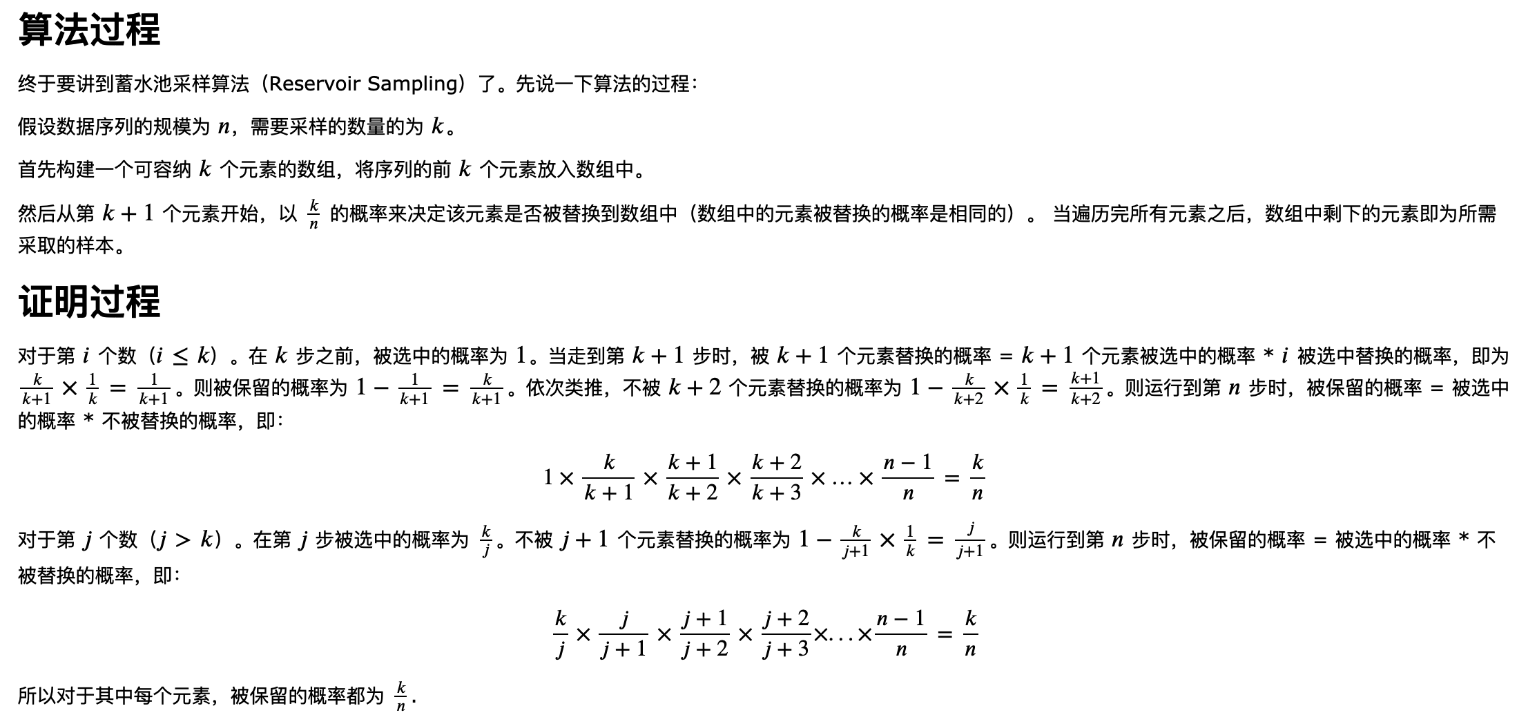
print(f"绝对误差: {abs(pi_estimate - 3.141592653589793)}")

蓄水池采样

与大模型关系不大，但是也记录一下。

import random
 
def reservior_sampling(n, k):
	nums = [i for i in range(1, n + 1)]
	res = []
	for i in range(k): # 直接填充前k个数字
		res.append(nums[i])
	for i in range(k + 1, len(nums)):
		# 此后每个新元素有k/i概率替换进去
		replace_idx = random.randint(0, i)
		if replace_idx < k:
			res[replace_idx] = nums[i]
	return res

🌨 云雪融

🍀探索

大模型从零开始（二）手撕代码

Shuffle 函数

Softmax 函数

MSE 损失

交叉熵损失

多头注意力机制 (MHA)

查询注意力机制 (MQA)

分组查询注意力机制 (GQA)

交叉注意力机制

Layer Normalization

RMS Normalization

MLP

Transformer Encoder

Transformer Decoder

位置编码

RoPE

LoRA

KL 散度

AUC 指标

梯度下降/牛顿法求平方根

GRPO Loss

InfoNCE

Focal Loss

蒙特卡洛估算圆周率

蓄水池采样

📇目录

🍀探索

🔀随便看看

花旗杯生存指南

日常工具使用记录

设计模式复习

🍀探索

大模型从零开始（二） 手撕代码

Shuffle 函数

Softmax 函数

MSE 损失

交叉熵损失

多头注意力机制 (MHA)

查询注意力机制 (MQA)

交叉注意力机制

Layer Normalization

RMS Normalization

MLP

Transformer Encoder

Transformer Decoder

位置编码

KL 散度

AUC 指标

梯度下降/牛顿法求平方根

Focal Loss

蒙特卡洛估算圆周率

蓄水池采样

📇目录

🍀探索

🔀随便看看

大模型从零开始（二）手撕代码